Introduction
A decision tree in general parlance represents a hierarchical series of binary decisions. A decision tree in machine learning works in exactly the same way, and except that we let the computer figure out the optimal structure & hierarchy of decisions, instead of coming up with criteria manually.
How a Decision Tree looks like
 Can you see how the model classifies a given input as a series of decisions? The tree is truncated here, but following any path from the root node down to a leaf will result in "Yes" or "No". Do you see how a decision tree differs from a logistic regression model?
How a Decision Tree is Created
Note the gini value in each box. This is the loss function used by the decision tree to decide which column should be used for splitting the data, and at what point the column should be split. A lower Gini index indicates a better split. A perfect split (only one class on each side) has a Gini index of 0.
Conceptually speaking, while training the models evaluates all possible splits across all possible columns and picks the best one. Then, it recursively performs an optimal split for the two portions. In practice, however, it's very inefficient to check all possible splits, so the model uses a heuristic (predefined strategy) combined with some randomization.
Decision Trees using Scikit-Learn
We can use DecisionTreeClassifier from sklearn.tree to train a decision tree.
Training
from sklearn.tree import DecisionTreeClassifier
model = DecisionTreeClassifier(random_state=50)
model.fit(X_train, train_targets)
Evaluation
Let's evaluate the decision tree using the accuracy_score.
from sklearn.metrics import accuracy_score, confusion_matrix
train_preds = model.predict(X_train)
train_preds

array(['No', 'No', 'No', ..., 'No', 'No', 'No'], dtype=object)
The decision tree also returns probabilities for each prediction.
train_probs = model.predict_proba(X_train)
train_probs

array([[1., 0.],
       [1., 0.],
       [1., 0.],
       ...,
       [1., 0.],
       [1., 0.],
       [1., 0.]])
Seems like the decision tree is quite confident about its predictions.
Let's check the accuracy of its predictions.
accuracy_score(train_targets, train_preds)

0.9999797955307714
The training set accuracy is close to 100%! But we can't rely solely on the training set accuracy, we must evaluate the model on the validation set too.
We can make predictions and compute accuracy in one step using model.score
model.score(X_val, val_targets)

0.7921188555510418
Although the training accuracy is 100%, the accuracy on the validation set is just about 79%, which is only marginally better than always predicting "No".
It appears that the model has learned the training examples perfectly, and doesn't generalize well to previously unseen examples. This phenomenon is called "overfitting", and reducing overfitting is one of the most important parts of any machine learning project.
Visualization
We can visualize the decision tree learned from the training data.
from sklearn.tree import plot_tree, export_text
plt.figure(figsize=(80,20))
plot_tree(model, feature_names=X_train.columns, max_depth=2, filled=True);

Let's check the depth of the tree that was created.
model.tree_.max_depth
We can also display the tree as text, which can be easier to follow for deeper trees.
tree_text = export_text(model, max_depth=10, feature_names=list(X_train.columns))
print(tree_text[:5000])
Feature Importance
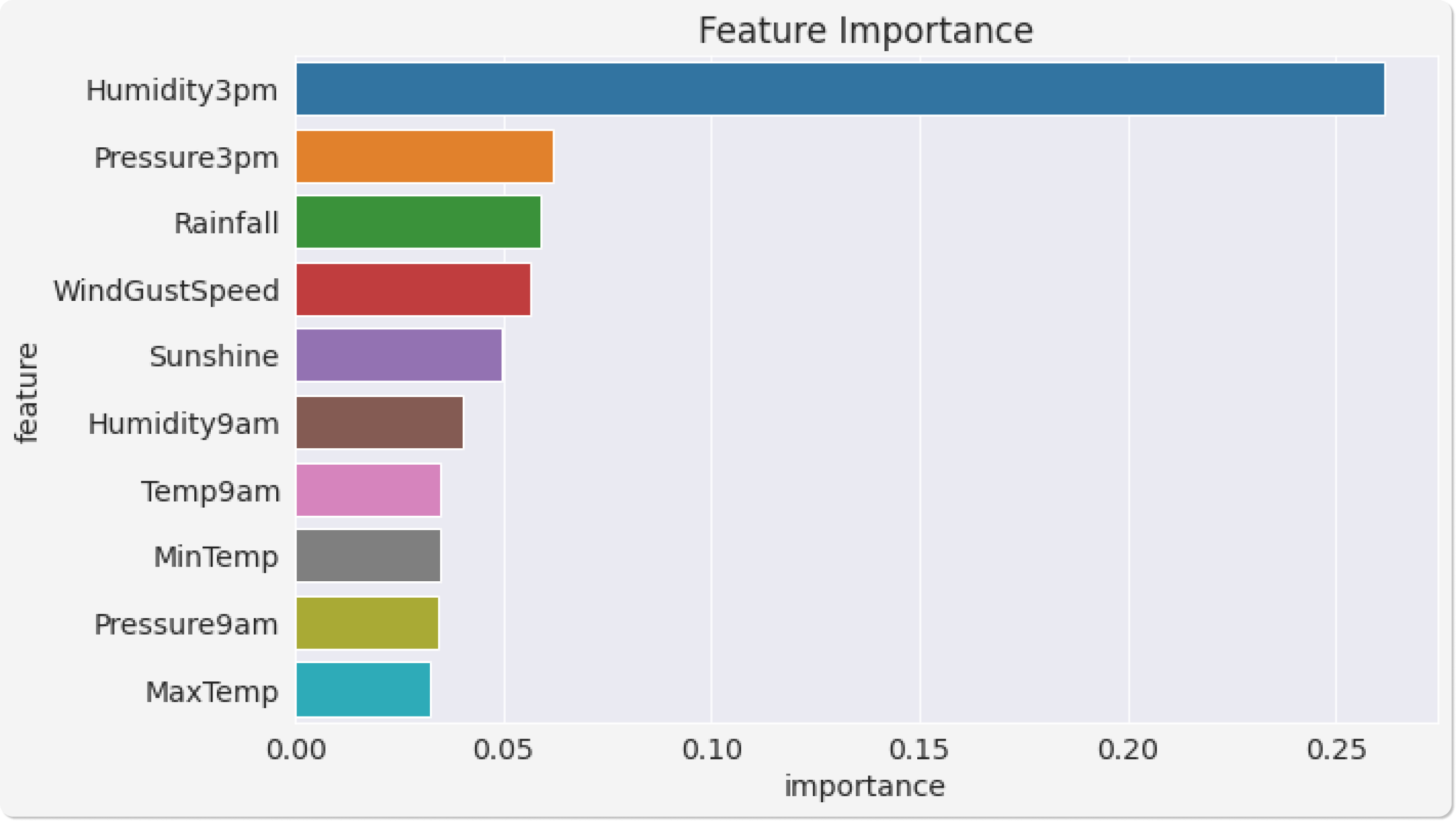
Based on the gini index computations, a decision tree assigns an "importance" value to each feature. These values can be used to interpret the results given by a decision tree.
model.feature_importances_

array([3.48942086e-02, 3.23605486e-02, 5.91385668e-02, 2.49619907e-02,
       4.94652143e-02, 5.63334673e-02, 2.80205998e-02, 2.98128801e-02,
       4.02182908e-02, 2.61441297e-01, 3.44145027e-02, 6.20573699e-02,
       1.36406176e-02, 1.69229866e-02, ...])
Let's turn this into a data frame and visualize the most important features.
importance_df = pd.DataFrame({
    'feature': X_train.columns,
    'importance': model.feature_importances_
}).sort_values('importance', ascending=False)
importance_df.head(10)
| feature | importance | |
| 9 | Humidity3pm | 0.261441 |
| 11 | Pressure3pm | 0.062057 |
| 2 | Rainfall | 0.059139 |
| 5 | WindGustSpeed | 0.056333 |
| 4 | Sunshine | 0.049465 |
| 8 | Humidity9am | 0.040218 |
| 14 | Temp9am | 0.035000 |
| 0 | MinTemp | 0.034894 |
| 10 | Pressure9am | 0.034415 |
| 1 | MaxTemp | 0.032361 |
plt.title('Feature Importance')
sns.barplot(data=importance_df.head(10), x='importance', y='feature');

Conclusion
In conclusion, decision trees are a powerful machine learning technique for both regression and classification. They are easy to interpret and explain, and they can handle both categorical and numerical data. However, decision trees can be prone to overfitting, especially when they are not pruned. If you are considering using decision trees for your machine learning project, be sure to keep this in mind. If you like this article, please consider sponsoring me. If you have any questions, please ask them in the comments or on Twitter. Thanks for reading!
